11. 微生物差异箱型图

微生物物种差异箱型图

11.1 tax_plot模块

tax_plot模块是可以根据4.1的data_filter函数筛选出各个级别的核心微生物并进行差异性分析可视化。

11.1.1 参数介绍

• data：

  由data_filter函数产生的包含各个样本微生物的数据框。

• tax_select

  指定需要进行差异性分析的物种。

• method

  指定差异分析的检验方法，包含T检验、onewayANOVA的多重检验(HSD, LSD,duncan,scheffe,REGW,SNK)。

• width_total

  指定全部物种汇总拼图的宽度

• height_total

  指定全部物种汇总拼图的高度

• width

  指定单独物种图形的宽度

• height

  指定单独物种图形的高度

• seed

  指定随机数种子，便于确定图形中散点的随机分布。【默认：123】

• group_level

  指定图形中分组显示的排列顺序。

• mytheme

  支持ggplot2主题代码，便于图形美化。

• palette

  指定绘图色板。

11.1.2 使用范例

代码示例：

# 首先利用过滤核心模块读取原始数据
library(EasyMicroPlot)  # 加载包
core_data <- data_filter(dir  = '16s_data/',design = 'mapping/mapping.txt',
                         min_relative = 0.001,min_ratio = 0.7)
# 选择出自己需要的微生物级别数据
sp <- core_data$filter_data$species
# 利用函数进行计算，这里选择V14,V15,V15用于示例
tax_re <- tax_plot(data = sp,tax_select = c('V14','V15','V16'),
                   method = 'LSD',width = 5,height = 5)

tax_re$pic # 这里存储了基本图形结果
tax_re$html # 这里存储交互式图形结果
tax_re$Post_Hoc # 当method选择onewayANOVA的多重检验时，这里存储了事后检验的详细结果

基本计算结果：

# 详细的时候多重事后检验结果
tax_re$Post_Hoc

$V14
          difference pvalue signif.           LCL         UCL
CT - ID -0.002209020 0.6419         -0.0118903818 0.007472342
CT - IO  0.007127541 0.1417         -0.0025538212 0.016808903
ID - IO  0.009336561 0.0581       . -0.0003448013 0.019017922

$V15
          difference pvalue signif.           LCL          UCL
CT - ID -0.003261756 0.1208         -0.0074471973 0.0009236855
CT - IO  0.004577676 0.0334       *  0.0003922346 0.0087631173
ID - IO  0.007839432 0.0007     ***  0.0036539905 0.0120248732

$V16
          difference pvalue signif.           LCL        UCL
CT - ID -0.002920911 0.5940         -0.0140806819 0.00823886
CT - IO  0.008443461 0.1315         -0.0027163101 0.01960323
ID - IO  0.011364372 0.0463       *  0.0002046009 0.02252414

图形结果展示：

# T检验结果
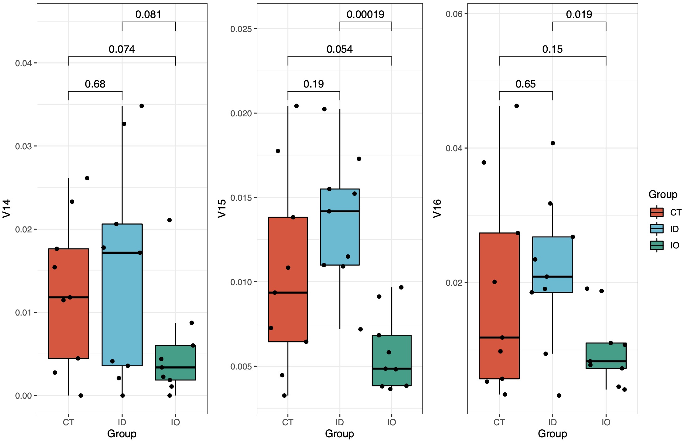
tax_re <- tax_plot(data = sp,tax_select = c('V14','V15','V16','V17'),method = 'ttest')
tax_re$pic$total

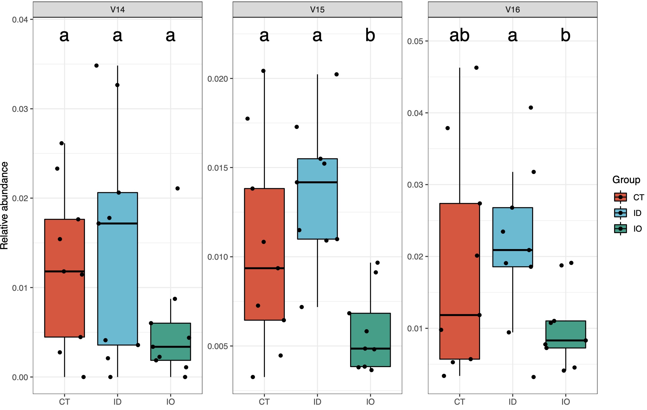
# onewayANOVA的多重检验
tax_re <- tax_plot(data = sp,tax_select = c('V14','V15','V16'),method = 'LSD')
tax_re$pic$total

# 结果也支持输出交互式图形，便于发现离群样本等情况
tax_re$html$total

Tips 1：可以将鼠标放在感兴趣的点，查询样本信息及基本情况。

# tax_plot支持ggplot2主题语法，可以使用mytheme参数进行进一步美化
library(ggplot2)
newtheme_slope=theme(axis.text.x =element_text(angle = 45, hjust = 1,size = 10)) # 例如调整分组名称的角度
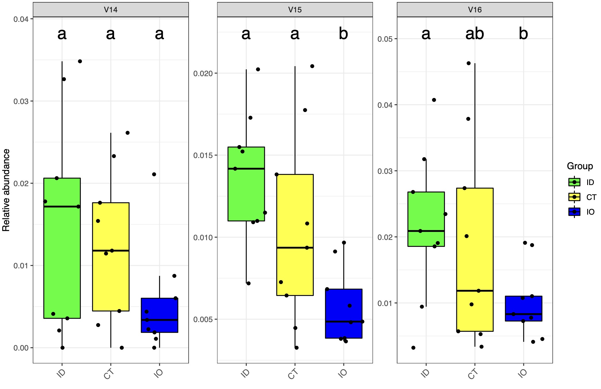
group_order <- c('ID','CT','IO') ## 设定排序，名称需要绝对一致
cols <- c('green','yellow','blue') ## 设定颜色方案
tax_re <- tax_plot(data = sp,tax_select = c('V14','V15','V16'),method = 'LSD',
                  mytheme = newtheme_slope)
tax_re$pic$total